Introduction
Almost all elementary statistics textbooks are broken up and ordered in the following way: Part 1: Descriptive Statistics, Part 2: Probability, and Part 3: Inferential Statistics (Bluman, 2017; Larson, 2022; Levin et al., 2016; Witte & Witte, 2017). The most powerful takeaway of an elementary statistics course is the inferential statistics portion found in Part 3. Generally speaking, students do well in Part 1, poorly in Part 2, and passable in Part 3. Probability is the necessary link between Parts 1 and 3 with the key takeaway being an understanding and familiarity with sampling distributions and how they apply towards statistical inference. With that said, probability is the most challenging part of the course. Resampling methods bridge Parts 1 and 3 without the challenges of learning all the details of probability. Once students learn about relative frequency histograms from Part 1, the thought is that they can more intuitively and easily understand sampling distributions produced by resampling methods (Chance et al., 2017; Tintle et al., 2018). The resampling approach is very direct and does not require a long sequence of classical probability, sampling distributions, and central limit theorem. A variety of current textbooks have taken the resampling approach (Lock et al., 2021; Tintle et al., 2020). Not only are resampling methods easier to understand, they have revolutionized statistics and are commonly used in practice (Bai & Pan, 2008; Bradley Efron’s Profile | Stanford Profiles, n.d.; Latpate et al., 2021; Yu, 2001).
The aim of this study is to compare the bootstrapping percentile method for estimating one sample proportion to methods traditionally taught in elementary statistics courses. In particular, for bootstrapping the percentile method will be compared to the Wald method, the plus 4 approximation of Agresti and Coull’s method, and the Clopper-Pearson “exact” method. The latter is not commonly introduced in elementary statistics textbooks but will serve as a comparison for small sample and edge cases where \(\widehat{p}\) is close to zero or one. All simulation, graphs, and tables in this study were produced using R.
Bootstrapping
The general idea of bootstrapping is to construct a sampling distribution based on the sample obtained. Once a sample is obtained, a computer is used to resample from the original sample with replacement. These resamples are referred to as bootstrap samples. For each bootstrap sample, the sample statistic of interest is calculated. This is called the bootstrap estimate. This procedure is repeated usually at least 1,000 times. Finally, the bootstrap estimates are sorted and used to construct a confidence interval.
Notation
\({\widehat{\theta}}^{*}\) is the bootstrapped estimate of \(\theta\) and \(\widehat{\theta}\) is the original sample estimate of \(\theta\). Similarly, \({\widehat{SE}}^{*}\) is an estimator of the standard error of \({\widehat{\theta}}^{*}\) and is calculated for each bootstrap sample. \(\widehat{SE}\) is an estimator of the standard error of \(\widehat{\theta}\) and is calculated from the original sample.
Percentile Method
There is a variety of ways to form confidence intervals by bootstrapping. The percentile method is the most straightforward and easiest to understand. Obtain R many bootstrap samples (usually at least 1,000) from the original sample and obtain the bootstrap estimates of interest. Then sort the bootstrap estimates and form an interval by using the cutoffs for the \(\frac{\alpha}{2}\) and \(1 - \frac{\alpha}{2}\) percentiles.
For instance, suppose you resample 1,000 times, compute 1,000 bootstrap estimates, and sort them in ascending order. Then you will have the following sorted array of estimates
\[\left\lbrack {\widehat{\theta}}_{1}^{*},\ {\widehat{\theta}}_{2}^{*},\ {\widehat{\theta}}_{3}^{*},\ldots,\ {\widehat{\theta}}_{998}^{*},\ {\widehat{\theta}}_{999}^{*},\ {\widehat{\theta}}_{1000}^{*} \right\rbrack\]
where \({\widehat{\theta}}_{1}^{*}, \leq {\widehat{\theta}}_{2}^{*} \leq {\widehat{\theta}}_{3}^{*} \leq \ldots \leq {\widehat{\theta}}_{1000}^{*}\). Now suppose you would like to compute a 95% confidence interval to estimate \(\theta\). You would form it by using \({\widehat{\theta}}_{25}^{*}\) as the lower limit and \({\widehat{\theta}}_{975}^{*}\) as the upper limit. In general, the percentile confidence interval looks like the following
\[\left( {\widehat{\theta}}_{\frac{\alpha}{2}}^{*},\ {\widehat{\theta}}_{1 - \frac{\alpha}{2}}^{*} \right)\]
For the purposes of this paper \(\theta = p = x/N\), is the population proportion, and \(\widehat{\theta} = \widehat{p} = X/n\), is the sample proportion, where \(X\sim binomial(n,\ p)\). The following are classical probability methods used in elementary statistics courses.
Wald
This is the standard classical approach to interval estimation for the population proportion \(p\).
\[\left( \widehat{p} - z_{1 - \frac{\alpha}{2}}\sqrt{\frac{\widehat{p}\left( 1 - \widehat{p} \right)}{n}},\ \widehat{p} + z_{1 - \frac{\alpha}{2}}\sqrt{\frac{\widehat{p}\left( 1 - \widehat{p} \right)}{n}} \right)\]
Adjusted Wald (Plus 4 approximation of Agresti Coull method for 95% confidence)
\[{\widehat{p}}_{a} = \frac{x + 2}{n + 4}\]
\[\left( {\widehat{p}}_{a} - 1.96\sqrt{\frac{{\widehat{p}}_{a}\left( 1 - {\widehat{p}}_{a} \right)}{n}},\ {\widehat{p}}_{a} + 1.96\sqrt{\frac{{\widehat{p}}_{a}\left( 1 - {\widehat{p}}_{a} \right)}{n}} \right)\]
The Clopper-Pearson “exact” method is usually not taught in an elementary statistics course, but it is shown here and will be used as a baseline for comparison in cases where \(n\) is small and/or \(\widehat{p}\) is close to zero or one.
\[\left( 1 + \frac{n - x + 1}{xF_{\frac{\alpha}{2},\ 2x,\ 2(n - x + 1)}},\ 1 + \frac{n - x}{(x + 1)F_{1 - \frac{\alpha}{2},\ 2(x + 1),\ 2(n - x)}} \right)\]
Methods
Samples from binomial distributions with varying sample sizes from \(n = 5\) to \(n = 1000\) and from \(p = 0.01\) to \(p = 0.99\) were simulated 1,000 times for each combination of \(n\) and \(p\). The tables in Appendix A show all levels used. Then, confidence intervals were constructed by the various methods listed. For each method, the number of times \(p\) was between the lower and upper bound of the interval was counted and divided by 1,000 to determine the coverage probability. For the bootstrap method, resampling was repeated 1,000 times. All confidence intervals were constructed with 95% confidence. All simulations were done using R.
Results
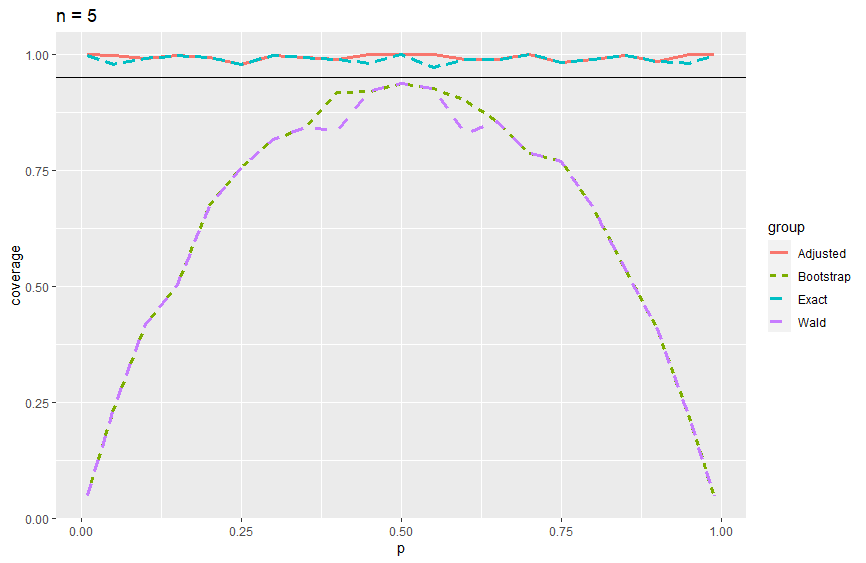
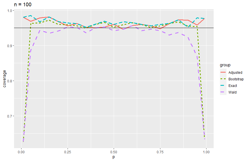
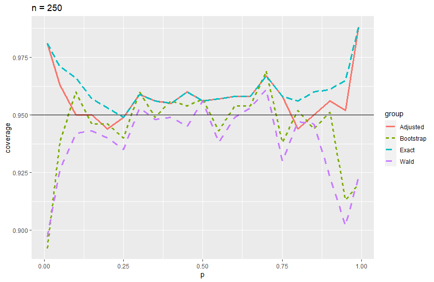
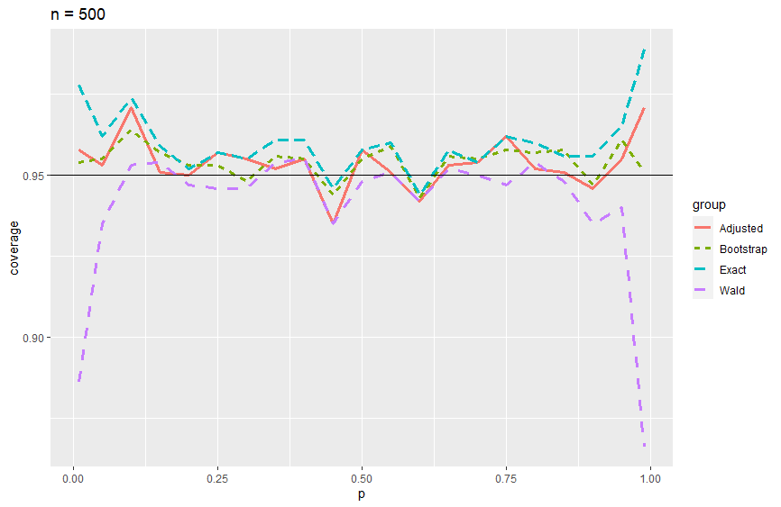
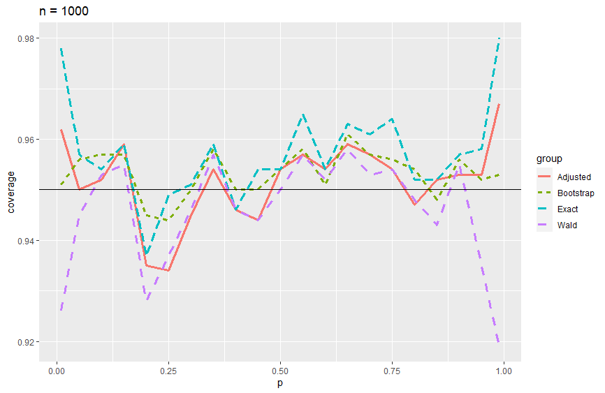
Coverage probability plots and tables (Appendix A) are presented to summarize the results. In the coverage probability plots, we see that the Wald and bootstrap methods mirror each other while the adjusted Wald and exact methods mirror each other as well. The Wald method performs poorly in the edge cases when \(p\) goes to 0 or 1 across all levels of \(n\) with improvements as \(n\) gets larger. The bootstrap method does this as well, but it stabilizes over all levels of \(p\) when \(n \geq 500\), giving consistent results around 95% coverage probability. Overall, the bootstrap percentile method performed at least as well as the Wald method when considering coverage probabilities. Where the bootstrap percentile method performed slightly better than the Wald method was for smaller sample sizes. In particular for sample sizes \(n = 5\) through \(n = 50\), we see that the bootstrap method performs a little better than the Wald method (Figures 1 through 4). Another important consideration is the average interval width. In terms of average interval width, the bootstrap and Wald methods performed nearly identically. For larger sample sizes, we see that the variability in interval widths was larger for the bootstrap method. Each cell in the tables found in Appendix A has, from left to right, coverage probability, average interval width, and the standard deviation of the interval width.
Conclusion
The bootstrap percentile method is very easy to understand and performs at least as well as the Wald method. The only time the Wald method had any advantage over the bootstrap was that it had better consistency (smaller standard deviation) in interval width when \(n \geq 250\). What the Wald method gave up to the bootstrap method in that range for \(n\) was coverage probability in the edge cases for \(p\). Resampling methods such as bootstrapping are commonly used and rely on very basic mathematics (Bai & Pan, 2008; Bradley Efron’s Profile | Stanford Profiles, n.d.; Latpate et al., 2021; Yu, 2001). One of the advantages that they bring to an elementary statistics course is a low barrier to understanding and to potentially improve student understanding of concepts and even retention (Tintle et al., 2018). Once a student gets through descriptive statistics, he or she does not need to know anything about probability and sampling distributions to comprehend the percentile method for bootstrapping confidence intervals. Furthermore, Recommendation 5: Use technology to explore concepts and analyze data from the GAISE College Report that states technology should aid student learning through the use of simulation (Chance et al., 2017). Another benefit of resampling methods is that the visualization of the sampling distribution becomes more concrete when it is obtained from data as opposed to an abstract distribution from mathematical statistics. The demystifying of sampling distributions can help students more intuitively understand important concepts such p-values. We also note that the performance of the bootstrap method in every relevant measure is comparable, if not better, than the Wald method. By adjusting the Wald method with the addition of 2 successes and 2 failures (plus 4 method) we see drastic improvement in the Wald method as noted by Agresti and Coull in their seminal 1998 paper, but students still need to spend weeks on learning probability and sampling distributions. In addition, adding 2 successes and 2 failures can seem arbitrary and mysterious to students as to why it makes such an improvement. At the very least, it is time that elementary statistics courses begin including resampling methods so students can gain familiarity with what is commonly used in practice (Bai & Pan, 2008; Bradley Efron’s Profile | Stanford Profiles, n.d.; Latpate et al., 2021; Yu, 2001).
Appendix
Figures and Tables from simulation results – The first number in tables is coverage probability, the second number is average interval width, and the third number is standard deviation of interval widths.

Figure 1.Coverage probability of 95% CI when n = 5.
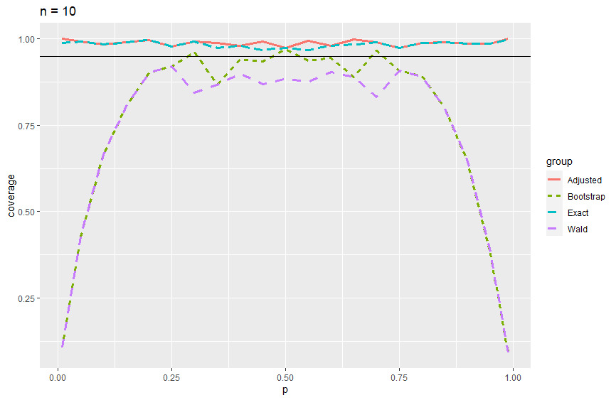
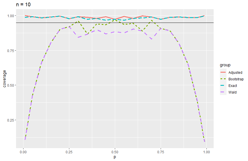
Figure 2.Coverage probability of 95% CI when n = 10.

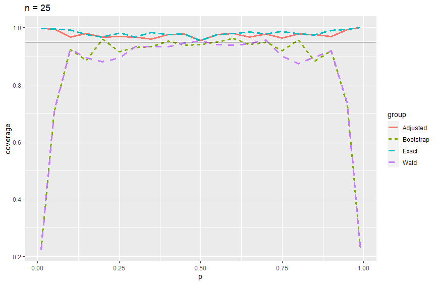
Figure 3.Coverage probability of 95% CI when n = 25.

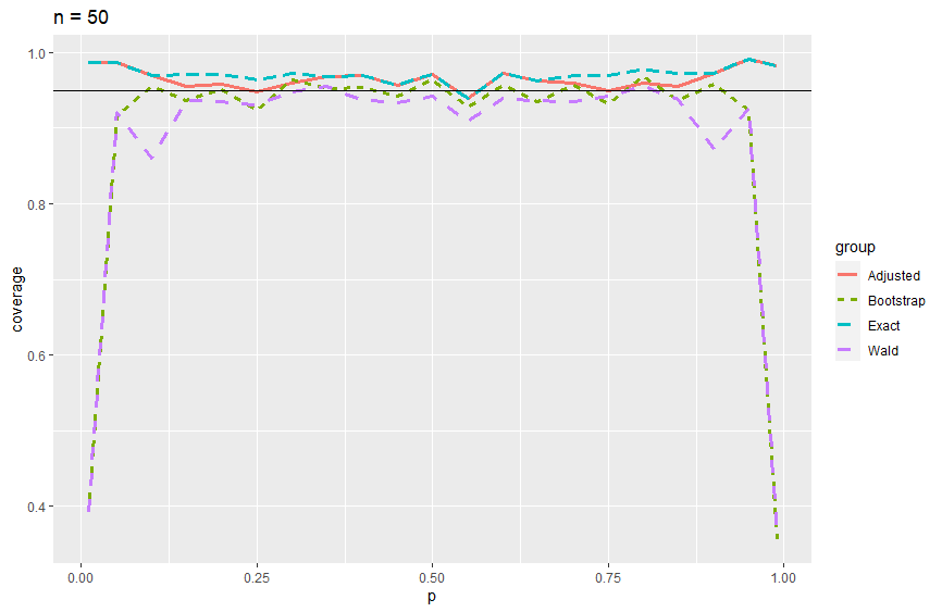
Figure 4.Coverage probability of 95% CI when n = 50.
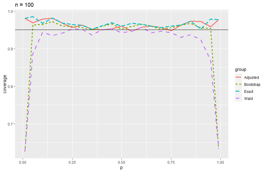
Figure 5.Coverage probability of 95% CI when n = 100.
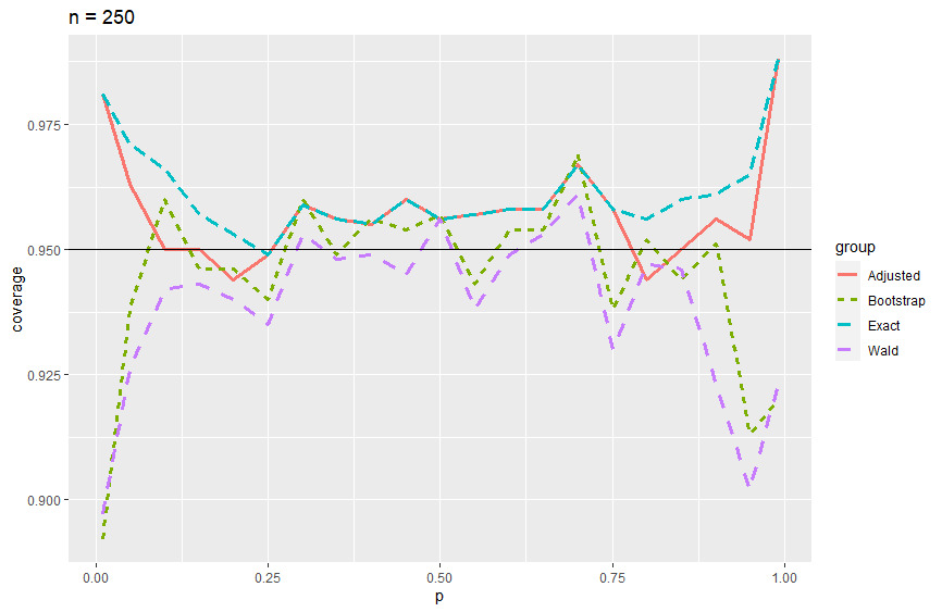
Figure 6.Coverage probability of 95% CI when n = 250.
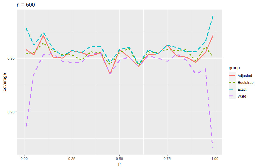
Figure 7.Coverage probability of 95% CI when n = 500.
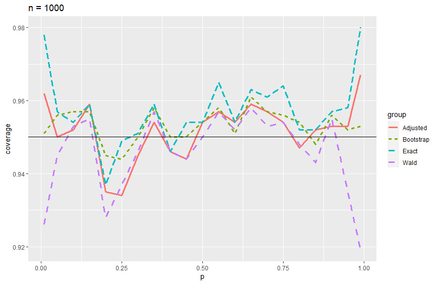
Figure 8.Coverage probability of 95% CI when n = 1000.
Table 1.Simulation Results (coverage probability, average width, standard deviation of widths).
| n = 5 |
|
|
|
|
| p |
Wald |
Adjusted |
Exact |
Bootstrap |
| 0.01 |
0.046(0.025)0.115 |
1.000(0.590)0.034 |
1.000(0.530)0.040 |
0.046(0.028)0.126 |
| 0.05 |
0.21(0.120)0.242 |
1.00(0.620)0.073 |
0.98(0.560)0.083 |
0.21(0.130)0.257 |
| 0.10 |
0.40(0.25)0.307 |
0.99(0.66)0.096 |
0.99(0.61)0.105 |
0.40(0.26)0.319 |
| 0.15 |
0.53(0.35)0.32 |
1.00(0.70)0.10 |
1.00(0.64)0.11 |
0.53(0.37)0.33 |
| 0.20 |
0.66(0.43)0.33 |
1.00(0.72)0.11 |
1.00(0.67)0.11 |
0.66(0.44)0.33 |
| 0.25 |
0.74(0.51)0.32 |
0.98(0.75)0.11 |
0.98(0.70)0.11 |
0.74(0.52)0.31 |
| 0.30 |
0.79(0.57)0.296 |
1.00(0.77)0.103 |
1.00(0.72)0.099 |
0.79(0.58)0.285 |
| 0.35 |
0.82(0.63)0.270 |
0.99(0.79)0.096 |
0.99(0.73)0.090 |
0.82(0.63)0.255 |
| 0.40 |
0.83(0.66)0.249 |
0.99(0.80)0.090 |
0.99(0.74)0.083 |
0.90(0.66)0.232 |
| 0.45 |
0.93(0.68)0.225 |
1.00(0.81)0.084 |
0.98(0.75)0.075 |
0.93(0.68)0.206 |
| 0.50 |
0.94(0.69)0.220 |
1.00(0.81)0.082 |
1.00(0.75)0.073 |
0.94(0.69)0.200 |
| 0.55 |
0.93(0.68)0.227 |
1.00(0.81)0.084 |
0.98(0.75)0.075 |
0.93(0.68)0.208 |
| 0.60 |
0.82(0.65)0.253 |
0.99(0.80)0.092 |
0.99(0.74)0.084 |
0.90(0.65)0.237 |
| 0.65 |
0.83(0.62)0.271 |
0.99(0.79)0.097 |
0.99(0.73)0.091 |
0.83(0.62)0.257 |
| 0.70 |
0.81(0.59)0.287 |
1.00(0.78)0.101 |
1.00(0.72)0.096 |
0.81(0.60)0.275 |
| 0.75 |
0.77(0.53)0.31 |
0.99(0.76)0.11 |
0.99(0.70)0.10 |
0.77(0.54)0.30 |
| 0.80 |
0.67(0.45)0.33 |
0.99(0.73)0.11 |
0.99(0.67)0.11 |
0.67(0.46)0.33 |
| 0.85 |
0.51(0.34)0.32 |
1.00(0.69)0.10 |
1.00(0.64)0.11 |
0.51(0.35)0.33 |
| 0.90 |
0.40(0.24)0.302 |
0.99(0.66)0.094 |
0.99(0.60)0.103 |
0.40(0.26)0.316 |
| 0.95 |
0.22(0.130)0.246 |
1.00(0.630)0.075 |
0.97(0.570)0.084 |
0.22(0.140)0.260 |
| 0.99 |
0.056(0.031)0.128 |
1.000(0.600)0.037 |
0.999(0.530)0.044 |
0.056(0.034)0.139 |
| Average |
0.61(0.44)0.265 |
0.99(0.73)0.090 |
0.99(0.67)0.089 |
0.62(0.44)0.262 |
Table 2.Simulation Results (coverage probability, average width, standard deviation of widths).
| n = 10 |
|
|
|
|
| p |
Wald |
Adjusted |
Exact |
Bootstrap |
| 0.01 |
0.10(0.030)0.090 |
1.00(0.370)0.035 |
0.99(0.320)0.043 |
0.10(0.032)0.095 |
| 0.05 |
0.39(0.13)0.165 |
0.99(0.41)0.068 |
0.99(0.37)0.080 |
0.39(0.13)0.176 |
| 0.10 |
0.69(0.25)0.187 |
0.99(0.46)0.080 |
0.99(0.43)0.092 |
0.69(0.26)0.197 |
| 0.15 |
0.80(0.32)0.189 |
0.99(0.49)0.082 |
0.99(0.47)0.095 |
0.80(0.34)0.198 |
| 0.20 |
0.89(0.40)0.179 |
0.99(0.53)0.078 |
0.99(0.51)0.091 |
0.89(0.42)0.182 |
| 0.25 |
0.92(0.45)0.165 |
0.98(0.55)0.071 |
0.98(0.53)0.084 |
0.92(0.47)0.163 |
| 0.30 |
0.82(0.49)0.144 |
1.00(0.57)0.061 |
1.00(0.55)0.074 |
0.96(0.50)0.139 |
| 0.35 |
0.88(0.53)0.116 |
0.99(0.58)0.049 |
0.98(0.57)0.061 |
0.89(0.54)0.109 |
| 0.40 |
0.90(0.56)0.090 |
0.98(0.60)0.037 |
0.98(0.59)0.048 |
0.95(0.56)0.083 |
| 0.45 |
0.85(0.57)0.077 |
0.99(0.60)0.032 |
0.96(0.59)0.042 |
0.93(0.57)0.070 |
| 0.50 |
0.89(0.58)0.068 |
0.97(0.60)0.028 |
0.97(0.60)0.037 |
0.96(0.58)0.062 |
| 0.55 |
0.86(0.57)0.077 |
0.99(0.60)0.031 |
0.97(0.60)0.042 |
0.95(0.57)0.068 |
| 0.60 |
0.92(0.57)0.083 |
0.99(0.60)0.034 |
0.99(0.59)0.045 |
0.95(0.57)0.076 |
| 0.65 |
0.89(0.54)0.109 |
1.00(0.59)0.046 |
0.99(0.58)0.058 |
0.89(0.54)0.102 |
| 0.70 |
0.83(0.50)0.136 |
0.99(0.57)0.058 |
0.99(0.56)0.071 |
0.96(0.51)0.131 |
| 0.75 |
0.92(0.45)0.163 |
0.98(0.55)0.070 |
0.98(0.53)0.083 |
0.92(0.46)0.161 |
| 0.80 |
0.89(0.41)0.177 |
0.99(0.53)0.077 |
0.99(0.51)0.089 |
0.89(0.42)0.179 |
| 0.85 |
0.78(0.33)0.196 |
0.99(0.50)0.085 |
0.99(0.47)0.098 |
0.78(0.34)0.203 |
| 0.90 |
0.63(0.23)0.196 |
0.99(0.46)0.084 |
0.99(0.42)0.096 |
0.63(0.25)0.207 |
| 0.95 |
0.42(0.14)0.168 |
0.99(0.41)0.070 |
0.99(0.37)0.081 |
0.41(0.14)0.180 |
| 0.99 |
0.10(0.030)0.089 |
1.00(0.370)0.035 |
0.99(0.320)0.042 |
0.10(0.031)0.094 |
| Average |
0.73(0.39)0.136 |
0.99(0.52)0.058 |
0.99(0.50)0.069 |
0.76(0.39)0.137 |
Table 3.Simulation Results (coverage probability, average width, standard deviation of widths).
| n = 25 |
|
|
|
|
| p |
Wald |
Adjusted |
Exact |
Bootstrap |
| 0.01 |
0.22(0.028)0.054 |
1.00(0.180)0.027 |
1.00(0.150)0.031 |
0.22(0.029)0.057 |
| 0.05 |
0.71(0.12)0.089 |
0.99(0.23)0.047 |
0.99(0.21)0.055 |
0.71(0.12)0.093 |
| 0.10 |
0.93(0.20)0.082 |
0.97(0.27)0.045 |
0.99(0.26)0.053 |
0.93(0.21)0.081 |
| 0.15 |
0.90(0.26)0.072 |
0.98(0.30)0.040 |
0.98(0.30)0.050 |
0.89(0.26)0.067 |
| 0.20 |
0.88(0.30)0.061 |
0.98(0.33)0.035 |
0.98(0.33)0.045 |
0.97(0.29)0.058 |
| 0.25 |
0.89(0.33)0.048 |
0.96(0.35)0.030 |
0.98(0.35)0.039 |
0.92(0.32)0.049 |
| 0.30 |
0.96(0.35)0.035 |
0.99(0.36)0.024 |
0.99(0.37)0.030 |
0.96(0.35)0.042 |
| 0.35 |
0.94(0.36)0.029 |
0.96(0.37)0.020 |
0.98(0.38)0.025 |
0.94(0.36)0.038 |
| 0.40 |
0.93(0.38)0.021 |
0.98(0.38)0.015 |
0.98(0.39)0.019 |
0.95(0.37)0.032 |
| 0.45 |
0.92(0.38)0.015 |
0.97(0.38)0.011 |
0.97(0.40)0.013 |
0.93(0.38)0.025 |
| 0.50 |
0.96(0.38)0.0117 |
0.96(0.39)0.0085 |
0.96(0.40)0.0105 |
0.95(0.39)0.0228 |
| 0.55 |
0.92(0.38)0.015 |
0.97(0.38)0.011 |
0.97(0.40)0.013 |
0.93(0.38)0.025 |
| 0.60 |
0.95(0.38)0.020 |
0.98(0.38)0.015 |
0.98(0.39)0.018 |
0.96(0.38)0.030 |
| 0.65 |
0.94(0.37)0.028 |
0.96(0.37)0.020 |
0.98(0.39)0.024 |
0.94(0.36)0.037 |
| 0.70 |
0.95(0.35)0.038 |
0.97(0.36)0.025 |
0.97(0.37)0.032 |
0.95(0.34)0.044 |
| 0.75 |
0.89(0.33)0.048 |
0.96(0.35)0.030 |
0.98(0.35)0.039 |
0.91(0.32)0.049 |
| 0.80 |
0.89(0.30)0.059 |
0.98(0.33)0.035 |
0.98(0.33)0.044 |
0.97(0.29)0.056 |
| 0.85 |
0.91(0.26)0.070 |
0.98(0.31)0.039 |
0.98(0.30)0.049 |
0.90(0.26)0.065 |
| 0.90 |
0.90(0.19)0.089 |
0.97(0.27)0.048 |
0.99(0.26)0.058 |
0.90(0.20)0.089 |
| 0.95 |
0.71(0.12)0.089 |
1.00(0.23)0.047 |
1.00(0.21)0.054 |
0.71(0.12)0.092 |
| 0.99 |
0.23(0.029)0.054 |
1.00(0.180)0.027 |
1.00(0.150)0.031 |
0.23(0.030)0.057 |
| Average |
0.84(0.28)0.049 |
0.98(0.32)0.029 |
0.98(0.32)0.035 |
0.85(0.28)0.053 |
Table 4.Simulation Results (coverage probability, average width, standard deviation of widths).
| n = 50 |
|
|
|
|
| p |
Wald |
Adjusted |
Exact |
Bootstrap |
| 0.01 |
0.38(0.026)0.035 |
0.99(0.100)0.019 |
0.99(0.087)0.022 |
0.38(0.027)0.037 |
| 0.05 |
0.92(0.10)0.046 |
0.99(0.15)0.028 |
0.99(0.14)0.032 |
0.91(0.10)0.046 |
| 0.10 |
0.87(0.16)0.039 |
0.96(0.18)0.026 |
0.96(0.18)0.032 |
0.95(0.16)0.038 |
| 0.15 |
0.94(0.19)0.031 |
0.95(0.21)0.023 |
0.97(0.21)0.027 |
0.94(0.19)0.031 |
| 0.20 |
0.93(0.22)0.025 |
0.95(0.23)0.020 |
0.97(0.23)0.024 |
0.94(0.21)0.027 |
| 0.25 |
0.94(0.24)0.020 |
0.95(0.24)0.017 |
0.96(0.25)0.019 |
0.93(0.23)0.023 |
| 0.30 |
0.92(0.25)0.016 |
0.95(0.26)0.014 |
0.97(0.27)0.015 |
0.96(0.25)0.020 |
| 0.35 |
0.95(0.26)0.012 |
0.97(0.26)0.010 |
0.97(0.27)0.011 |
0.95(0.26)0.018 |
| 0.40 |
0.95(0.27)0.0092 |
0.97(0.27)0.0078 |
0.97(0.28)0.0088 |
0.96(0.27)0.0151 |
| 0.45 |
0.93(0.27)0.0057 |
0.95(0.27)0.0048 |
0.95(0.29)0.0054 |
0.94(0.27)0.0126 |
| 0.50 |
0.94(0.27)0.0036 |
0.97(0.27)0.0030 |
0.97(0.29)0.0034 |
0.96(0.27)0.0108 |
| 0.55 |
0.94(0.27)0.0053 |
0.95(0.27)0.0045 |
0.95(0.29)0.0051 |
0.94(0.27)0.0124 |
| 0.60 |
0.92(0.27)0.0095 |
0.96(0.27)0.0081 |
0.96(0.28)0.0091 |
0.94(0.27)0.0154 |
| 0.65 |
0.95(0.26)0.0115 |
0.97(0.26)0.0098 |
0.97(0.28)0.0109 |
0.95(0.26)0.0166 |
| 0.70 |
0.93(0.25)0.017 |
0.95(0.26)0.014 |
0.97(0.26)0.016 |
0.96(0.25)0.021 |
| 0.75 |
0.93(0.24)0.021 |
0.94(0.24)0.017 |
0.96(0.25)0.020 |
0.93(0.23)0.023 |
| 0.80 |
0.93(0.22)0.025 |
0.95(0.23)0.020 |
0.97(0.23)0.023 |
0.95(0.22)0.026 |
| 0.85 |
0.94(0.19)0.029 |
0.96(0.21)0.022 |
0.98(0.21)0.026 |
0.94(0.19)0.030 |
| 0.90 |
0.90(0.16)0.038 |
0.97(0.18)0.025 |
0.97(0.18)0.030 |
0.97(0.16)0.036 |
| 0.95 |
0.92(0.10)0.046 |
0.99(0.15)0.027 |
0.99(0.14)0.032 |
0.92(0.11)0.046 |
| 0.99 |
0.44(0.030)0.036 |
0.98(0.110)0.020 |
0.98(0.089)0.022 |
0.44(0.031)0.038 |
| Average |
0.88(0.20)0.023 |
0.96(0.22)0.016 |
0.97(0.22)0.019 |
0.89(0.20)0.026 |
Table 5.Simulation Results (coverage probability, average width, standard deviation of widths).
| n = 100 |
|
|
|
|
| p |
Wald |
Adjusted |
Exact |
Bootstrap |
| 0.01 |
0.63(0.024)0.021 |
0.98(0.060)0.013 |
0.98(0.052)0.014 |
0.63(0.025)0.022 |
| 0.05 |
0.89(0.082)0.021 |
0.97(0.097)0.015 |
0.98(0.095)0.017 |
0.96(0.081)0.020 |
| 0.10 |
0.94(0.12)0.016 |
0.98(0.12)0.013 |
0.97(0.13)0.015 |
0.96(0.11)0.017 |
| 0.15 |
0.94(0.14)0.014 |
0.98(0.14)0.012 |
0.98(0.15)0.013 |
0.97(0.14)0.015 |
| 0.20 |
0.94(0.16)0.012 |
0.97(0.16)0.010 |
0.97(0.16)0.011 |
0.96(0.15)0.013 |
| 0.25 |
0.95(0.17)0.0098 |
0.96(0.17)0.0090 |
0.96(0.18)0.0096 |
0.96(0.17)0.0120 |
| 0.30 |
0.95(0.18)0.0081 |
0.96(0.18)0.0074 |
0.96(0.19)0.0079 |
0.96(0.18)0.0106 |
| 0.35 |
0.94(0.19)0.0060 |
0.95(0.19)0.0055 |
0.95(0.19)0.0058 |
0.95(0.18)0.0089 |
| 0.40 |
0.95(0.19)0.0041 |
0.95(0.19)0.0037 |
0.96(0.20)0.0039 |
0.96(0.19)0.0082 |
| 0.45 |
0.95(0.19)0.0024 |
0.95(0.19)0.0022 |
0.97(0.20)0.0024 |
0.97(0.19)0.0076 |
| 0.50 |
0.94(0.20)0.0014 |
0.96(0.20)0.0013 |
0.96(0.20)0.0014 |
0.95(0.19)0.0073 |
| 0.55 |
0.95(0.19)0.0025 |
0.95(0.19)0.0023 |
0.97(0.20)0.0024 |
0.96(0.19)0.0077 |
| 0.60 |
0.96(0.19)0.0041 |
0.96(0.19)0.0037 |
0.96(0.20)0.0040 |
0.96(0.19)0.0084 |
| 0.65 |
0.94(0.19)0.0062 |
0.96(0.19)0.0057 |
0.96(0.19)0.0061 |
0.96(0.18)0.0089 |
| 0.70 |
0.95(0.18)0.0082 |
0.96(0.18)0.0075 |
0.96(0.19)0.0080 |
0.95(0.18)0.0104 |
| 0.75 |
0.94(0.17)0.0099 |
0.95(0.17)0.0090 |
0.96(0.18)0.0096 |
0.96(0.17)0.0115 |
| 0.80 |
0.93(0.16)0.012 |
0.96(0.16)0.011 |
0.96(0.16)0.012 |
0.96(0.15)0.013 |
| 0.85 |
0.94(0.14)0.013 |
0.97(0.14)0.012 |
0.97(0.15)0.013 |
0.97(0.14)0.015 |
| 0.90 |
0.92(0.12)0.016 |
0.97(0.12)0.014 |
0.95(0.13)0.016 |
0.95(0.11)0.017 |
| 0.95 |
0.87(0.081)0.022 |
0.96(0.097)0.015 |
0.98(0.094)0.018 |
0.95(0.081)0.021 |
| 0.99 |
0.63(0.025)0.022 |
0.98(0.060)0.013 |
0.98(0.052)0.015 |
0.63(0.026)0.023 |
| Average |
0.91(0.15)0.0110 |
0.96(0.15)0.0088 |
0.97(0.16)0.0097 |
0.93(0.14)0.0132 |
Table 6.Simulation Results (coverage probability, average width, standard deviation of widths).
| n = 250 |
|
|
|
|
| p |
Wald |
Adjusted |
Exact |
Bootstrap |
| 0.01 |
0.92(0.021)0.0096 |
0.99(0.032)0.0062 |
0.99(0.029)0.0071 |
0.92(0.021)0.0095 |
| 0.05 |
0.93(0.053)0.0071 |
0.96(0.057)0.0064 |
0.97(0.058)0.0069 |
0.94(0.053)0.0075 |
| 0.10 |
0.93(0.074)0.0062 |
0.96(0.076)0.0059 |
0.97(0.078)0.0061 |
0.95(0.074)0.0070 |
| 0.15 |
0.94(0.088)0.0054 |
0.95(0.089)0.0051 |
0.96(0.092)0.0053 |
0.95(0.088)0.0063 |
| 0.20 |
0.95(0.099)0.0047 |
0.95(0.100)0.0046 |
0.96(0.100)0.0047 |
0.95(0.098)0.0057 |
| 0.25 |
0.94(0.11)0.0038 |
0.97(0.11)0.0037 |
0.97(0.11)0.0038 |
0.95(0.11)0.0052 |
| 0.30 |
0.94(0.11)0.0032 |
0.95(0.11)0.0031 |
0.95(0.12)0.0032 |
0.95(0.11)0.0049 |
| 0.35 |
0.95(0.12)0.0023 |
0.96(0.12)0.0023 |
0.96(0.12)0.0023 |
0.95(0.12)0.0045 |
| 0.40 |
0.95(0.12)0.0016 |
0.96(0.12)0.0015 |
0.96(0.12)0.0016 |
0.95(0.12)0.0042 |
| 0.45 |
0.95(0.12)0.00088 |
0.96(0.12)0.00086 |
0.96(0.13)0.00087 |
0.95(0.12)0.00414 |
| 0.50 |
0.96(0.12)0.00031 |
0.96(0.12)0.00030 |
0.96(0.13)0.00030 |
0.96(0.12)0.00401 |
| 0.55 |
0.95(0.12)0.00081 |
0.97(0.12)0.00078 |
0.97(0.13)0.00080 |
0.96(0.12)0.00419 |
| 0.60 |
0.95(0.12)0.0016 |
0.96(0.12)0.0015 |
0.96(0.12)0.0016 |
0.96(0.12)0.0042 |
| 0.65 |
0.95(0.12)0.0024 |
0.96(0.12)0.0023 |
0.96(0.12)0.0023 |
0.96(0.12)0.0045 |
| 0.70 |
0.95(0.11)0.0032 |
0.96(0.11)0.0031 |
0.96(0.12)0.0032 |
0.95(0.11)0.0049 |
| 0.75 |
0.94(0.11)0.0039 |
0.95(0.11)0.0038 |
0.95(0.11)0.0039 |
0.94(0.11)0.0052 |
| 0.80 |
0.95(0.099)0.0048 |
0.96(0.100)0.0046 |
0.96(0.100)0.0047 |
0.95(0.098)0.0059 |
| 0.85 |
0.95(0.088)0.0055 |
0.95(0.090)0.0052 |
0.96(0.092)0.0054 |
0.95(0.088)0.0062 |
| 0.90 |
0.94(0.074)0.0062 |
0.96(0.076)0.0058 |
0.97(0.078)0.0061 |
0.96(0.074)0.0067 |
| 0.95 |
0.92(0.053)0.0073 |
0.96(0.057)0.0066 |
0.98(0.058)0.0071 |
0.94(0.053)0.0077 |
| 0.99 |
0.93(0.021)0.0096 |
0.98(0.032)0.0062 |
0.98(0.029)0.0071 |
0.92(0.022)0.0095 |
| Average |
0.94(0.093)0.0043 |
0.96(0.095)0.0038 |
0.96(0.097)0.0040 |
0.95(0.093)0.0058 |
Table 7.Simulation Results (coverage probability, average width, standard deviation of widths).
| n = 500 |
|
|
|
|
| p |
Wald |
Adjusted |
Exact |
Bootstrap |
| 0.01 |
0.87(0.017)0.0045 |
0.97(0.020)0.0033 |
0.99(0.020)0.0038 |
0.96(0.017)0.0043 |
| 0.05 |
0.94(0.038)0.0036 |
0.95(0.039)0.0035 |
0.96(0.040)0.0036 |
0.96(0.038)0.0039 |
| 0.10 |
0.94(0.052)0.0032 |
0.95(0.053)0.0031 |
0.96(0.054)0.0032 |
0.96(0.052)0.0036 |
| 0.15 |
0.95(0.063)0.0027 |
0.95(0.063)0.0027 |
0.96(0.064)0.0027 |
0.96(0.062)0.0033 |
| 0.20 |
0.95(0.070)0.0023 |
0.95(0.070)0.0023 |
0.96(0.072)0.0023 |
0.96(0.070)0.0031 |
| 0.25 |
0.96(0.076)0.0019 |
0.97(0.076)0.0019 |
0.97(0.078)0.0019 |
0.97(0.075)0.0032 |
| 0.30 |
0.95(0.080)0.0016 |
0.95(0.080)0.0016 |
0.95(0.082)0.0016 |
0.95(0.080)0.0030 |
| 0.35 |
0.95(0.084)0.0012 |
0.95(0.084)0.0011 |
0.96(0.085)0.0012 |
0.95(0.083)0.0027 |
| 0.40 |
0.95(0.086)0.00077 |
0.95(0.086)0.00076 |
0.95(0.088)0.00077 |
0.95(0.085)0.00285 |
| 0.45 |
0.95(0.087)0.00042 |
0.95(0.087)0.00041 |
0.96(0.089)0.00041 |
0.95(0.087)0.00278 |
| 0.50 |
0.95(0.088)0.00012 |
0.95(0.088)0.00012 |
0.95(0.089)0.00012 |
0.95(0.087)0.00272 |
| 0.55 |
0.94(0.087)0.00043 |
0.94(0.087)0.00043 |
0.96(0.089)0.00043 |
0.95(0.087)0.00279 |
| 0.60 |
0.95(0.086)0.00080 |
0.95(0.086)0.00078 |
0.96(0.088)0.00079 |
0.95(0.085)0.00287 |
| 0.65 |
0.95(0.083)0.0012 |
0.95(0.084)0.0012 |
0.95(0.085)0.0012 |
0.95(0.083)0.0028 |
| 0.70 |
0.95(0.080)0.0016 |
0.96(0.080)0.0016 |
0.96(0.082)0.0016 |
0.95(0.080)0.0029 |
| 0.75 |
0.94(0.076)0.0020 |
0.95(0.076)0.0020 |
0.95(0.078)0.0020 |
0.95(0.075)0.0031 |
| 0.80 |
0.94(0.070)0.0023 |
0.94(0.070)0.0023 |
0.95(0.072)0.0023 |
0.95(0.070)0.0032 |
| 0.85 |
0.95(0.063)0.0027 |
0.95(0.063)0.0027 |
0.95(0.064)0.0027 |
0.95(0.062)0.0034 |
| 0.90 |
0.94(0.052)0.0031 |
0.96(0.053)0.0030 |
0.97(0.054)0.0031 |
0.95(0.052)0.0036 |
| 0.95 |
0.94(0.038)0.0035 |
0.96(0.039)0.0033 |
0.97(0.040)0.0034 |
0.96(0.038)0.0037 |
| 0.99 |
0.86(0.017)0.0047 |
0.96(0.020)0.0035 |
0.98(0.019)0.0040 |
0.94(0.016)0.0045 |
| Average |
0.94(0.066)0.0021 |
0.95(0.067)0.0020 |
0.96(0.068)0.0021 |
0.95(0.066)0.0033 |
Table 8.Simulation Results (coverage probability, average width, standard deviation of widths).
| n = 1000 |
|
|
|
|
| p |
Wald |
Adjusted |
Exact |
Bootstrap |
| 0.01 |
0.92(0.012)0.0021 |
0.95(0.013)0.0018 |
0.97(0.013)0.0020 |
0.95(0.012)0.0021 |
| 0.05 |
0.94(0.027)0.0018 |
0.95(0.027)0.0018 |
0.95(0.028)0.0018 |
0.95(0.027)0.0020 |
| 0.10 |
0.94(0.037)0.0016 |
0.94(0.037)0.0016 |
0.94(0.038)0.0016 |
0.94(0.037)0.0021 |
| 0.15 |
0.95(0.044)0.0014 |
0.95(0.044)0.0014 |
0.95(0.045)0.0014 |
0.96(0.044)0.0019 |
| 0.20 |
0.95(0.050)0.0012 |
0.95(0.050)0.0012 |
0.95(0.051)0.0012 |
0.96(0.049)0.0020 |
| 0.25 |
0.95(0.054)0.00098 |
0.95(0.054)0.00097 |
0.96(0.055)0.00097 |
0.95(0.053)0.00197 |
| 0.30 |
0.95(0.057)0.00079 |
0.95(0.057)0.00078 |
0.96(0.058)0.00079 |
0.95(0.056)0.00199 |
| 0.35 |
0.96(0.059)0.00057 |
0.96(0.059)0.00057 |
0.96(0.060)0.00057 |
0.96(0.059)0.00185 |
| 0.40 |
0.94(0.061)0.0004 |
0.94(0.061)0.0004 |
0.94(0.062)0.0004 |
0.94(0.060)0.0019 |
| 0.45 |
0.95(0.062)0.0002 |
0.95(0.062)0.0002 |
0.96(0.063)0.0002 |
0.96(0.061)0.0019 |
| 0.50 |
0.95(0.062)0.00004 |
0.96(0.062)0.00004 |
0.96(0.063)0.00004 |
0.96(0.062)0.00193 |
| 0.55 |
0.94(0.062)0.00021 |
0.94(0.062)0.00020 |
0.94(0.063)0.00020 |
0.95(0.061)0.00190 |
| 0.60 |
0.94(0.061)0.0004 |
0.95(0.061)0.0004 |
0.95(0.062)0.0004 |
0.95(0.060)0.0020 |
| 0.65 |
0.94(0.059)0.00059 |
0.94(0.059)0.00059 |
0.95(0.060)0.00059 |
0.95(0.059)0.00189 |
| 0.70 |
0.95(0.057)0.00080 |
0.95(0.057)0.00079 |
0.95(0.058)0.00080 |
0.96(0.056)0.00192 |
| 0.75 |
0.94(0.054)0.00098 |
0.95(0.054)0.00097 |
0.96(0.055)0.00098 |
0.95(0.053)0.00190 |
| 0.80 |
0.95(0.050)0.0012 |
0.95(0.050)0.0012 |
0.95(0.050)0.0012 |
0.95(0.049)0.0019 |
| 0.85 |
0.95(0.044)0.0013 |
0.95(0.044)0.0013 |
0.95(0.045)0.0013 |
0.95(0.044)0.0019 |
| 0.90 |
0.95(0.037)0.0016 |
0.94(0.037)0.0016 |
0.95(0.038)0.0016 |
0.95(0.037)0.0020 |
| 0.95 |
0.95(0.027)0.0018 |
0.94(0.027)0.0017 |
0.95(0.028)0.0018 |
0.95(0.027)0.0020 |
| 0.99 |
0.93(0.012)0.0020 |
0.96(0.013)0.0018 |
0.97(0.013)0.0019 |
0.95(0.012)0.0021 |
| Average |
0.95(0.047)0.0010 |
0.95(0.047)0.0010 |
0.95(0.048)0.0010 |
0.95(0.047)0.0020 |